1004: Priciples of Economics (3)
Chapter 4: The market forces of Demand and Supply:
Chapetr 6: Supply, Demand and Governement Policies
What is demand? Draw a demand curve with a demand scedule. What are the determinants of demand? (5)
What is supply? Draw a supply curve with a supply schedule. What are the determinants of Supply? (5)
Define the equilibrium of a market. Describe the forces that move a market towards its equlibrium.
When does market equilibrium occur? show in Figure. (2.5)
a) Draw and explain a production possibilities frontier for an economy that produces computers and cars.(5.5)
b) What is the demand curve? Discuss at least two variables that can shift the demand curve.(3.5)
c) What is the supply curve? Discuss at least two variables that can shift the supply curve.(3.5)
1004 Exam Paper- Section A; 2015-16 (Click to see the Exam paper)
Chapter 7: Consumers, Producers and the efficiency of Markets
Chpeter 8: Application: The Costs of Taxation
What happens to consumer and producer surplus when the sale of good is taxed? Explain.
Draw a supply and demand diagram with a tax on the sale of the good. Show the deadweight loss and tax revenue.
What happens to deadweight loss and tax revenue when a tax is increased? Draw the figure and explain.
What does the “Invisible Hand“ of the marketplace do? Explain the two main causes of market failure and give an example of each.
… … …
Define negative externality with relevant examples.(3)
what are the corrective taxes? Why do economists prefer them to regulations as a way to protect the environment from pollution? Discuss (2+7.5)
Question Notes- Handmades with Graph and schedule.
-
Chapter 04- The Market Fources of Demand and Supply:
Market, Market Fources, Competetion (1-3)
Demand, Quantity Demanded, Law of Demand, demand Curve, Demand Schedule (4-8)
Movement along the curve, Shifts of the demand curve, Increase in Demand, Decrease in Demand, Variables that influences buyer.(9-13)
Supply: Supply Curve, Quantity Supplied, Law of Supply, Supply Schedule, Supply Curve, movement along the supply curve, shifts of the supply curve,Variables that influnences Sellers.(14-21)
Supply and Demand Curve together: Equilibrium, Equilibrium Price, Equilibrium Quantity, Surplus, Shortages, There steps of analysing changes in Equlibrium. (22-28)
Chapter 05: The Elasticities and Its application
The Elascity of Demand
The Elasticity of Supply
Three Applications of Supply, Demand and Elasticity.
Chapter 6: Supply, Demand and Governement Policies
The Surprising effects of Price Controls
The Surprising effects of Tax Incidence
Conclusion
Chapter 7: Consumers, Producers and the Efficieny of Market Prices:
Consumer Surplus
Producer Surplus
Market Efficiency
Conclusion: Market Efficiency and Market Failure
Chpater 8: Application: The Cost of Taxation
The deadweight loss of taxation
The determinants of Deadwight Loss
DWL and Tax Revenue as Taxes Vary
Conclusion:
-
Chpater 4: The Market Fources of Supply and Demand:
◆ Economists use the model of supply and demand to analyze competitive markets. In a competitive market, there are many buyers and sellers, each of whom has little or no influence on the market price.
◆ The demand curve shows how the quantity of a good demanded depends on the price. According to the law of demand, as the price of a good falls, the quantity demanded rises. Therefore, the demand curve slopes downward.
◆ In addition to price, other determinants of the quantity demanded includeincome, tastes, expectations, and the prices of substitutes and complements. If one of these other determinants changes, the demand curve shifts.
◆ The supply curve shows how the quantity of a good supplied depends on the price. According to the law of supply, as the price of a good rises, the quantity supplied rises. Therefore, the supply curve slopes upward.
◆ In addition to price, other determinants of the quantity supplied include input prices, technology, and expectations. If one of these other determinants changes, the supply curve shifts.
◆ The intersection of the supply and demand curves determines the market equilibrium.At the equilibrium price, the quantity demanded equals the quantity supplied.
◆ The behavior of buyers and sellers naturally drives markets toward their equilibrium. When the market price is above the equilibrium price, there is a surplus of the good, which causes the market price to fall. When the market price is below the equilibrium price, there is a shortage, which causes the market price to rise.
◆ To analyze how any event influences a market, we use the supply-and-demand diagram to examine how the event affects the equilibrium price and quantity. To do this we follow three steps.
First, we decide whether the event shifts the supply curve or the demand curve (or both).
Second, we decide which direction the curve shifts.
Third, we compare the new equilibrium with the old equilibrium.
◆ In market economies, prices are the signals that guide economic decisions and thereby allocate scarce resources. For every good in the economy, the price ensures that supply and demand are in balance. The equilibrium price then determines how much of the good buyers choose to purchase and how much sellers choose to produce.
……………………………………………
-
Chapter 5: Elasticity and Its Application:
◆ The price elasticity of demand measures how much the quantity demanded responds to changes in the price. Demand tends to be more elastic if the good is a luxury rather than a necessity, if close substitutes are available, if the market is narrowly defined, or if buyers have substantial time to react to a price change.
◆ The price elasticity of demand is calculated as the percentage change in quantity demanded divided by the percentage change in price. If the elasticity is less than 1, so that quantity demanded moves proportionately less than the price, demand is said to be inelastic. If the elasticity is greater than 1, so that quantity demanded moves proportionately more than the price, demand is said to be elastic.
◆ Total revenue, the total amount paid for a good, equals the price of the good times the quantity sold. For inelastic demand curves, total revenue rises as price rises. For elastic demand curves, total revenue falls as price rises.
◆ The income elasticity of demand measures how much the quantity demanded responds to changes in consumers’ income. The cross-price elasticity of demand measures how much the quantity demanded of one good responds to the price of another good.
◆ The price elasticity of supply measures how much the quantity supplied responds to changes in the price. This elasticity often depends on the time horizon under consideration. In most markets, supply is more elastic in the long run than in the short run.
◆ The price elasticity of supply is calculated as the percentage change in quantity supplied divided by the percentage change in price. If the elasticity is less than 1, so that quantity supplied moves proportionately less than the price, supply is said to be inelastic. If the elasticity is greater than 1, so that quantity supplied moves proportionately more than the price, supply is said to be elastic.
◆ The tools of supply and demand can be applied in many different kinds of markets. This chapter uses them to analyze the market for wheat, the market for oil, and the market for illegal drugs.
……………………………………………
-
Chapter 6: Supply, Demand and Government Policies
◆ A price ceiling is a legal maximum on the price of a good or service. An example is rent control. If the price ceiling is below the equilibrium price, the quantity demanded exceeds the quantity supplied. Because of the resulting shortage, sellers must in some way ration the good or service among buyers.
◆ A price floor is a legal minimum on the price of a good or service. An example is the minimum wage. If the price floor is above the equilibrium price, the quantity supplied exceeds the quantity demanded. Because of the resulting surplus, buyers’ demands for the good or service must in some way be rationed among sellers.
◆ When the government levies a tax on a good, the equilibrium quantity of the good falls. That is, a tax on a market shrinks the size of the market.
◆ A tax on a good places a wedge between the price paid by buyers and the price received by sellers. When the market moves to the new equilibrium, buyers pay more for the good and sellers receive less for it. In this sense, buyers and sellers share the tax burden. The incidence of a tax does not depend on whether the tax is levied on buyers or sellers.
◆ The incidence of a tax depends on the price elasticities of supply and demand. The burden tends to fall on the side of the market that is less elastic because that side of the market can respond less easily to the tax by changing the quantity bought or sold.
……………………………………………
-
Chapter 7: Consumers, Producers and the Efficiency of Markets
◆ Consumer surplus equals buyers’ willingness to pay for a good minus the amount they actually pay for it, and it measures the benefit buyers get from participating in a market. Consumer surplus can be computed by finding the area below the demand curve and above the price.
◆ Producer surplus equals the amount sellers receive for their goods minus their costs of production, and it measures the benefit sellers get from participating in a market. Producer surplus can be computed by finding the area below the price and above the supply curve.
◆ An allocation of resources that maximizes the sum of consumer and producer surplus is said to be efficient. Policymakers are often concerned with the efficiency, as well as the equity, of economic outcomes.
◆ Under Normal Condition, The equilibrium of supply and demand maximizes the sum of consumer and producer surplus. That is, the invisible hand of the marketplace leads buyers and sellers to allocate resources efficiently.
◆ Markets do not allocate resources efficiently in the presence of market failures such as market power or externalities.
……………………………………………
-
Chapter 8: Application: The Cost of Taxation
◆ A tax on a good reduces the welfare of buyers and sellers of the good, and the reduction in consumer and producer surplus usually exceeds the revenue raised by the government. The fall in total surplus—the sum of consumer surplus, producer surplus, and tax revenue— is called the deadweight loss of the tax.
◆ Taxes have deadweight losses because they cause buyers to consume less and sellers to produce less, and this change in behavior shrinks the size of the market below the level that maximizes total surplus. Because the elasticities of supply and demand measure how much market participants respond to market conditions, larger elasticities imply larger deadweight losses.
◆ As a tax grows larger, it distorts incentives more, and its deadweight loss grows larger. Tax revenue first rises with the size of a tax. Eventually, however, a larger tax reduces tax revenue because it reduces the size of the market.
……………………………………………
Chapter 04: The market Forces of Supply and Demand
4.2: Demand:
Quantity Demanded: the amount of a good that buyers are willing and able to purchase.
Law of Demand: the claim that, other things being equal, the quantity demanded of a good falls when the price of the good rises. (figure1)
Variables and their effect:
A changes in the price represents a movement along the demand curve. (fig 1, pp 64)
A change in one of the other variables shifts the demand curve. (fig 3, pp 66)
Determinants of Quantity Demanded:
Central variable: Price
Other variables:
Income (normal goods and Inferior Goods),
Prices of related goods (Substitutes and Complements),
Tastes,
Expectations,
Number of Buyers.
Demand Schedule: a table that shows the relationship between the price of a good and the quantity demanded
Demand Curve: a graph of the relationship between the price of a good and the quantity demanded
Market demand: is the sum of individual demand. (fig 2, pp65)
4.2c) Shifts in the Demand curve:
Increase in demand = Shift the demand curve to the right.
Decrease in demand = Shift the demand curve to the left
Normal Good: A good for which, other things being equal, an increase in income leads to an increase in demands. (Icecreams)
Inferior Good: A good for which, other things being equal, an increase in income leads to a decrease in demands. (Bus rides)
Substitute: Two goods for which an increase in price of one leads to an increase in demands for the others. (Tea and Coffee)
Complements: Two goods for which an increase in price of one leads to an decrease in demands for the others. (Car and fuel)
4.3: Supply
Quantity Supplied: The amount of a good that sellers are willing and able to sell.
Law of Supply: The claim that, other things being equal, the quantity supplied of a good rises when the price of a good rises.
Supply Schedule: A table that shows the relationship between the price of a good and quantity supplied.
Supply Curve: A graph of the relationship between price of a good and the quantity suplied.
Market Suppy versus Individual Supply: MS is the sum of All IS.
Shifts in the supply Curve: (Figure 7)
Increase in supply = shifts the curve to the right (When the quantity increases)
Decrease the supply = shifts the curve to the left (when the quantity decreases)
Effects of the Variables:
Main variable: Price
Other Variables: Input Prices, Technology, Expectations, Number of Sellers.
Change in the price = Movement along the Supply Curve (fig 5)
Changes in the non-price factors = Shift the supply curve. (fig 7)
Table: Determinants of Demand and Supply
| Determinants of Demand | Determinants of Supply |
|---|---|
| 1. Price of Goods 2. Income of Consumers 3. Prices of Related Goods 4. Tastes and Preferences 5. Number of Buyers 6. Expectations |
1. Price of Goods: 2. Cost of Production 3. Prices of Related Goods in Production 4. Technology 5. Number of Sellers 6. Governement Policies 7. Expectations |
4.4. Supply and Demand Together:
Equilibrium: a situation in which the market price has reached the level at which the quantity supplied equals the quantity demanded.
Equilibrium Price: the price that balances the quantity demanded and quantity supplied.
Equilibrium Quantity: the quantity supplied and quantity demanded at the equlibrium price.
Surplus: A situation in which quantity supplied is gretaer than the quantity demanded. (when price rises)
Shortages: A situation in which the quantity demanded is greater than the quantity Supplied. (When price falls)
Law of Supply and Demand: The claim that the price of any good adjusts to bring the quantity supplied and the quantity demanded of that good into balance.
Question: Define the equilibrium of a market. Describe the forces that move a market towards its equlibrium.
Answer:
In economics, a market reaches equilibrium when the quantity of a good or service that consumers are willing and able to buy equals the quantity that producers are willing and able to sell.
At this intersection, the market is "cleared," meaning there is no inherent tendency for the price or the quantity to change unless an external force shifts supply or demand.
1. The Equilibrium Components
To understand how a market stabilizes, we look at three key variables:
Equilibrium Price ($P^*$): Also known as the market-clearing price; the price where the plans of buyers and sellers match.
Equilibrium Quantity ($Q^*$): The amount of the good bought and sold at the equilibrium price.
The Law of Supply and Demand: This dictates that as price increases, demand falls and supply rises, and vice versa.
2. Forces Moving the Market Toward Equilibrium
If a market is not at equilibrium, it faces either a surplus or a shortage. Market forces—specifically the "Invisible Hand" of self-interest and price flexibility—act as corrective mechanisms.
A. Correcting a Surplus (Excess Supply)
A surplus occurs when the current market price is above the equilibrium price.
The Situation: At this high price, producers want to sell more than consumers want to buy
The Correction: Warehouses fill with unsold goods. To clear this inventory, competing sellers lower their prices. As the price drops, two things happen:
Consumers increase their quantity demanded.
Producers decrease their quantity supplied.
Result: The price continues to fall until it reaches to the equilibrium price
B. Correcting a Shortage (Excess Demand)
A shortage occurs when the current market price is below the equilibrium price.
The Situation: At this low price, consumers want to buy more than producers are willing to provide.
The Correction: Buyers, unable to find the product, offer to pay higher prices to secure what is available. Sellers, seeing the high demand, realize they can raise prices without losing customers. As the price rises:
Producers are incentivized to supply more.
Some consumers drop out of the market, reducing quantity demanded.
Result: The price continues to rise until it reaches to the equlibrium price.
Summary Table: Market Adjustments
| Market Condition | Price vs. Equilibrium | Result | Pressure on Price |
|---|---|---|---|
| Surplus | $P > P^*$ | $Q_s > Q_d$ | Downward (Sellers cut prices) |
| Equilibrium | $P = P^*$ | $Q_s = Q_d$ | Neutral (Market is stable) |
| Shortage | $P < P^*$ | $Q_d > Q_s$ | Upward (Buyers bid prices up) |
What specific market or industry are you currently looking at to see these forces in action?
3 steps for analysing the changes in equilibrium: (fig 10) ***
If the event shifts the supply or demand curve or both
Decide in which direction of the curve shifts
use a supply and demand diagram to see how the shift changes equlibrium price and quantity.
Figure 8: The equlibrium of Supply and Demand:
The market equlibrium is where the supply and demand curve intersect.
Figure 9: Markets not in equlibrium:
(Surplus and Shortages)
Figure 10: How an increase in demand affects the equlibrium:
both equlibrium price and equlibrium quantity increase.
Figure 11: How a decrease in a supply affects the equlibrium:
Equlibrium price rise, equlibrium quantity falls
Figure 12: A shifts in both Supply and Demand
two possible outcomes:
Equilibrium Price and Equilibrium quantity, both, rises.
Equilibrium Price rises and Equilibrium quantity falls.
Table 4: Whats happens to Price and Quantity and when supply or demand shifts?
| No change in Supply | An Increase in Supply | A decrease in Supply | |
|---|---|---|---|
| No chane in Demand | P same Q same |
P down Q up |
P up Q down |
| An Increase in Demand | P up Q up |
P ambiguous Q Up |
P up Q ambiguous |
| A decrease in Demand | P down Q down |
P down Q ambiguous |
P ambiguous Q down |
Chapter: 06: Supply, Demand and Government Policies
[Key words: Price Ceiling and Price Floor. ]
The economy is governed by two kinds of laws: The law of supply and demands and the laws enacted by governement. Such two instruments for govt for market control are: Price Ceiling and Price Floor.
Price Ceiling= A legal maximum on the price at which a good can be sold.
Price Floor = A legal minimum on the price at which a good can be sold.
6.1) Surprising Effects of Price Controls: Two effect may create
6.1 (a) Effects of Price Ceiling: (two effects)
A) Icecreams: (figure 1)
Price ceiling above the equilibrium price = has no binding effect = market can reach the equilibrium of supply and demands = quantity supplied equals quantity demanded.
Price ceiling below the equilibrium price = has binding effect= causes market ‘shortages’ = sellers must ration scarce goods = Causes Long lines= Efficient
A) Gasoline: (figure 2)
Price ceiling above the equilibrium price = has no binding effect = market can reach the equilibrium of supply and demands = quantity supplied equals quantity demanded.
Price ceiling below the equilibrium price = has binding effect= causes market ‘shortages’ = sellers must ration scarce goods = Causes Long lines= Inefficient
A) Rent Controls: (figure 3)
Short Run = Supply and Demand curve for apartments inelastic = Causes a small shortage of Apartments
Long run = Supply and Demand curve for apartments more elastic = causes a larger shortages of Apartments
Effects of Price Floors: Two effects
A market with a price floor (figure 4):
The floor pricing is lower the equlibrium price = No Binding Effect = Reaches a new equilibrium where the quantity demanded and quantity Supplied are equals.
The floor pricing is above the equlibrium price = Surplus arises.
Minimum Wages: (Figure 5)
A Free Labor Market: reaches an equlibrium
A labor market with a binding minimum wages = Price Floor = Causes Surplus = Labor Supplied exceeds the qunatity Demanded = The result is unemployment.
6.2) The surprising Effects of Tax Incidence:
When the government levies a tax on a good, the Equilibrium qunatity of the good falls, that is, a tax on a market shrinks the market’s size.
Tax on a good = Equilibrium quantity falls = market size shrinks.
The incidence of a Tax on a good = Equilibrium moves = buyers pay more = seller receives less = Buyers and sellers share the tax burden = So, it is not the matter whether the tax is levied on the buyers or sellers.
The incidence of a tax = depends on the the price elasticities of supply and demand.
Figure 6: A tax on Sellers
Buyers and Sellers share the burden
Figure 7: A Tax on Buyers
Buyers and Sellers share the burden
Figure 9: How a tax burden is divided
the supply curve is elastic and the demand curve is inelastic = Buyers bear most of the tax burden.
the supply curve is inelastic and the demand curve is elastic = Sellers bear most of the Tax burden
Chapter: 07: Consumers, Producers and the efficiency of Markets
Consumer Surplus: The amount a buyer is willing to pay minus the amount the buyer is actually pays for it.
Lower prises raises the Consumer Surplus.
Consumer Surplus reflects economic wellbeing.
Buyers are rational when they make decisions.
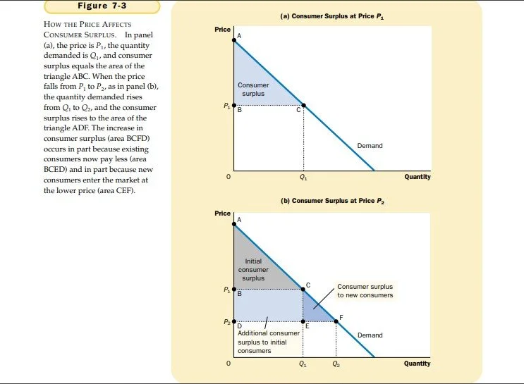
Fig 3: How price affects the consumer Surplus, pp137
Producer Surplus: The amount a seller is paid for a good minus the seller’s cost of providing it.
Higher prices raises the Producers Surplus.
Producer Surplus measure the wellbeing of the sellers.
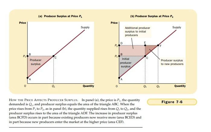
Fig 6: How price affects the Producer Surplus, pp 142
Market Efficiency:
Total surplus: TS is the area between the supply and demand curves up to the equilibrium quantity.
Societal Wellbeing = Consumer Surplus + Producer Surplus
Consumer Surplus + Producer Surplus = Total Surplus.
Total Surplus is the natural variable for the social planners.
If the total Surplus becomes maximum= The resources exhibits Efficiency.
Competitive Markets:
allocate the supply of goods to the buyers who value them most.
allocate the demand for goods to the sellers who can produce them at the lowest cost.
produce the quantity of goods that maximises the sum of consumer and producer surplus.
Under normal Conditions, the equlibrium of supply and demand maximises the total surplus (as the invisible hand in the marketplace causes the markets to allocate resources efficiently).
The Market equilibrium maximises the sum of producer and consumer surplus. (Fig 7.8; see below)
Markets do not allocate resources efficiently in the presence of market failure such as market power or externalities.
Efficiency: the property of a resource allocation of maximizing the total surplus received by all members of society
Equity: the fairness of the distribution of well-being among the members of society
These observations lead to two insights about market outcomes:
Free markets allocate the supply of goods to the buyers who value them most highly, as measured by their willingness to pay.
Free markets allocate the demand for goods to the sellers who can produce them at least cost.
Thus, given the quantity produced and sold in a market equilibrium, the social planner cannot increase economic well-being by changing the allocation of consumption among buyers or the allocation of production among sellers. But can the social planner raise total economic well-being by increasing or decreasing the quantity of the good?
The answer is no, as stated in this third insight about market outcomes:
Free markets produce the quantity of goods that maximizes the sum of consumer and producer surplus.
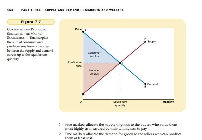
Fig 7: Consumer Surplus and Producer Surplus in the Market Equlibrium, pp 144
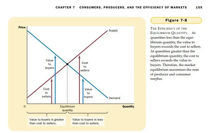
Fig 8: The Efficiency of the Equlibrium Quantity, pp145
Qestion: What does the “Invisible Hand“ of the marketplace do? Explain the two main causes of market failure and give an example of each.
Answer:
The "Invisible Hand" is a metaphor introduced by Adam Smith in The Wealth of Nations. It describes the unintended social benefits resulting from individual self-interest.
In a well-functioning market, individuals looking to maximize their own profit or utility are led, as if by an "invisible hand," to promote the efficient allocation of resources. For instance, a baker doesn't produce bread out of pure altruism; they do it to earn a living. However, to earn that living, they must produce bread that is high quality and reasonably priced, which ultimately benefits the consumer and society at large.
Market Failure
Market failure occurs when the "Invisible Hand" fails to allocate resources efficiently on its own, leading to a loss of social welfare. Economists generally categorize the causes into two main areas:
1. Externalities
An externality occurs when the production or consumption of a good affects a third party who is not involved in the transaction. Because the market price does not reflect these "hidden" costs or benefits, the market produces too much or too little of the good.
Example:Pollution (Negative Externality). A factory producing steel may dump waste into a nearby river. The cost of cleaning the water or the health impact on the local community isn't paid by the factory or the steel buyer. Consequently, the price of steel is artificially low, leading to overproduction and excessive pollution.
2. Market Power (Monopoly/Oligopoly)
Market failure also happens when a single buyer or seller (or a small group) has the ability to exert significant influence over market prices. This prevents the forces of supply and demand from reaching a natural equilibrium.
Example:A Life-Saving Medication (Monopoly). If one pharmaceutical company holds a patent on a unique, life-saving drug and faces no competition, they can restrict the quantity produced and charge a price far above the cost of production. This results in "deadweight loss," where many people who need the drug cannot afford it, even though it would be efficient for them to have it.
Summary Table:
| Cause of Failure | Mechanism | Market Outcome |
|---|---|---|
| Externalities | Side effects on bystanders are ignored. | Over-consumption (negative) or under-consumption (positive). |
| Market Power | One player controls price or supply. | Prices are too high; quantity is too low. |
Would you like to explore how governments typically intervene to correct these specific types of failures?
Chapter: 08: The Cost of Taxation
Tax a good= Allocation of Resources Less Efficient= Distort Incentives = Create a deadweight Loss= Reduces the welfare of Buyers and Sellers = Reduction in consumer surplus and Producer Surplus exceeds the revenues raised.
As a Tax grows larger= distorts incentives more = deadweight Loss grow larger = reduces the size of the market = tax revenue starts to fall.
Tax revenue first rises with size of the tax = but if the tax gets large enough, Tax revenue starts to Fail
Determinants of DWL= Price elasticities of demand and supply.
The greater the elasticities of the demand and supply and demand, the larger the deadweight loss of tax.
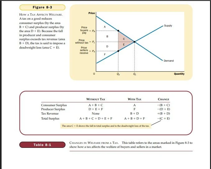
Figure-3: How a TAx Affects Welfare
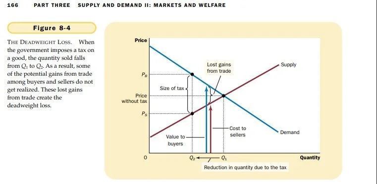
Fig 4: The sources of Deadweight Loss
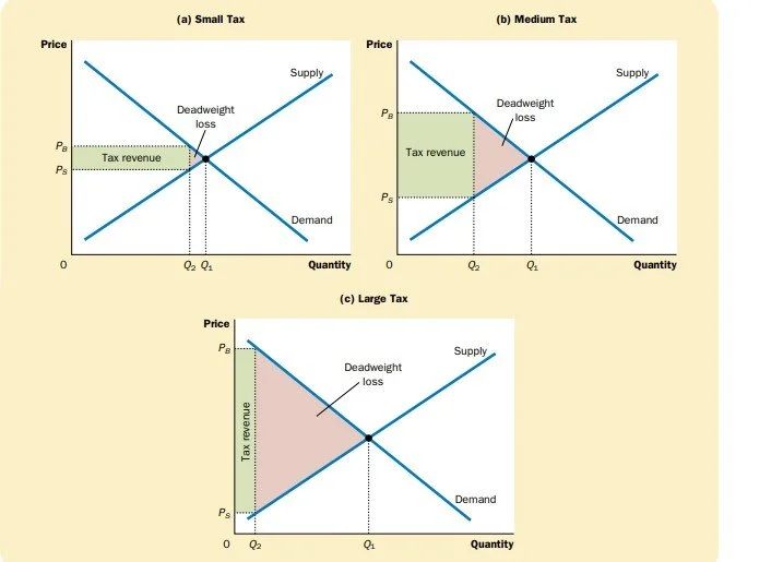
Fig 6: How Deadweight Loss and Tax Revenue Vary with the size of a Tax (part 1)
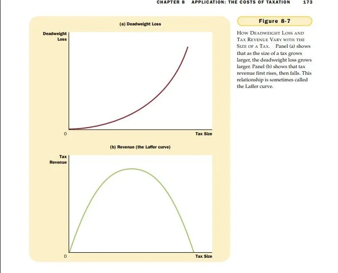
Fig 6: How Deadweight Loss and Tax Revenue Vary with the size of a Tax. (part 2)
